1. Implementing and Comparing ODE Methods#
We implemented and compared three numerical methods for solving ordinary differential equations (ODEs).
1.1. Numerical Methods#
1.1.1. Explicit Euler#
1.1.2. Implicit Euler#
1.1.3. Improved Euler (Heun’s Method)#
1.2. Test Problem#
To investigate the long-time stability of these methods, we solve the second-order ODE
which describes a simple harmonic oscillator.
Rewriting it as a first-order system yields
The exact solution conserves the total energy
making this problem well suited for studying numerical stability and energy conservation.
1.3. Numerical Results#
The following plots show the behavior of the numerical solutions for larger time intervals:
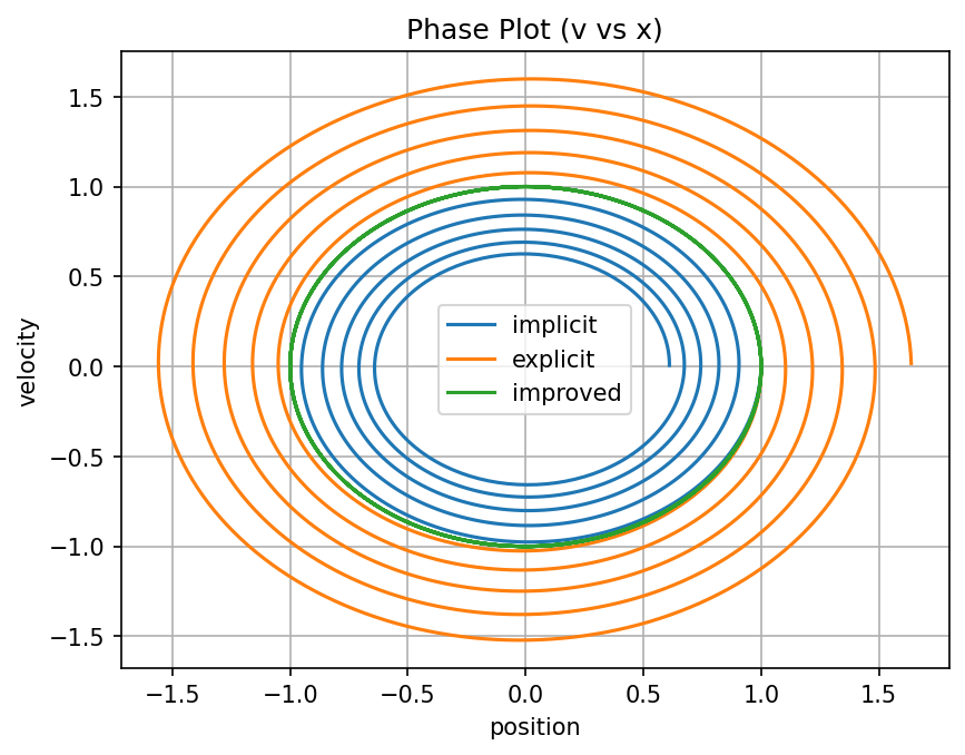
Phase portrait: velocity vs. position
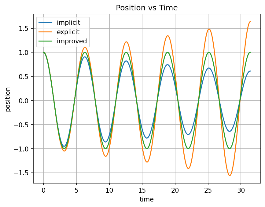
Position vs. time
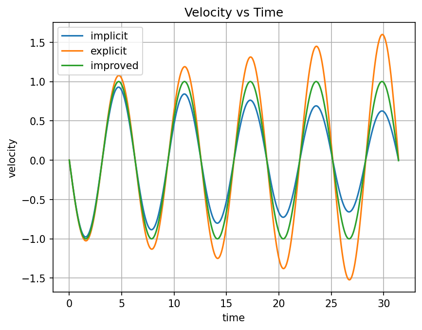
Velocity vs. time
1.3.1. Phase Portrait#
1.3.2. Position vs. Time#
1.3.3. Velocity vs. Time#
1.4. Discussion#
The plots indicate that:
The explicit Euler method adds energy to the system, leading to an unstable spiral in phase space.
The implicit Euler method removes energy, causing the solution to decay over time.
The improved Euler method conserves energy much better and closely reproduces the expected periodic motion.