2. Perfectly Matched Layers (PML) in NGSolve#
This notebook provides a comprehensive introduction to Perfectly Matched Layers (PML) in the frequency domain and demonstrates their implementation using NGSolve/Netgen.
We begin by exploring NGSolve’s built-in Cartesian PML functionality, which provides an elegant solution for absorbing boundary conditions in wave propagation problems.
from ngsolve import *
from netgen.occ import *
from ngsolve.webgui import Draw
import numpy as np
import matplotlib.pyplot as plt
2.1. Geometry Setup#
The computational domain consists of:
Interior region: A square where the physical problem is solved
PML region: Surrounding layers that will absorb outgoing waves
This layered structure allows us to simulate wave propagation in an effectively infinite domain while using a finite computational mesh.
def create_geo():
    rect_outer = MoveTo(-2,-2).Rectangle (4,4).Face()
    rect_outer.edges.name = 'outerbnd'

    rec1 = MoveTo(-1, -2).Rectangle(2,1).Face()
    rec2 = MoveTo(-1, 1).Rectangle(2, 1).Face()
    rec3 = MoveTo(1, -1).Rectangle(1,2).Face()
    rec4 = MoveTo(-2, -1).Rectangle(1,2).Face()

    quad1 = MoveTo(1,1).Rectangle(1,1).Face()
    quad2 = MoveTo(-2,1).Rectangle(1,1).Face()
    quad3 = MoveTo(1,-2).Rectangle(1,1).Face()
    quad4 = MoveTo(-2,-2).Rectangle(1,1).Face()
    rect = MoveTo(-1,-1).Rectangle(2,2).Face()

    Rectangles = Glue([rec1, rec2, rec3, rec4, quad1, quad2, quad3, quad4])
    pml_region = Rectangles - rect
    pml_region.faces.name = 'pmlregion'


    geo = Glue([rect, pml_region])
    return geo

mesh = Mesh(OCCGeometry(create_geo(), dim=2).GenerateMesh(maxh=0.2))
2.2. PML Implementation in NGSolve#
In NGSolve, PMLs are implemented as mesh transformations that apply complex coordinate scaling. The Cartesian PML creates a complex scaling transformation outside a specified rectangular region.
The complex scaling effectively “stretches” the coordinates in the complex plane, causing waves to decay exponentially as they propagate through the PML region.
In Chapter 3 of the Bachelor Thesis we see how the corresponding comlex scaled system looks like. In ngsolve those computations are internally done in the pml class with additional mesh transformation.
pml_cart = pml.Cartesian((-1,-1),(1,1),alpha = 2j)
mesh.SetPML(pml_cart,'.*')
The NGsolve PML class allows to access the scaling and its Jacobian and determinant as a CoefficientFunction
Draw(pml_cart.PML_CF.real,mesh,vectors=True)
Draw(pml_cart.PML_CF.imag,mesh,vectors=True)

#Draw(pml_cart.Det_CF.real,mesh)
#Draw(pml_cart.Det_CF.imag,mesh)

#Draw(pml_cart.Jac_CF.real,mesh)
#Draw(pml_cart.Jac_CF.imag,mesh)
BaseWebGuiScene
2.3. Helmholtz Equation with PML#
We will now solve the Helmholtz equation:
\(-\Delta u - \omega^2 u = f\).
Note that the complex scaled Helmholtz solution only satisfies this equation in the interior (unscaled) domain.
f_0 = exp(-4**2*((x-0.2)**2+(y-0.2)**2))
def solve_PML(mesh, order = 5):
    fes = H1(mesh, order=order, complex=True, )
    u = fes.TrialFunction()
    v = fes.TestFunction()

    omega = 10

    a = BilinearForm(fes)
    a += grad(u)*grad(v)*dx - omega**2*u*v*dx
    #a += -1j*omega*u*v*ds("outerbnd")   #neumann BD at the outerbnd
    a.Assemble()

    f = LinearForm(f_0 * v * dx).Assemble()

    gfu = GridFunction(fes)
    gfu.vec.data = a.mat.Inverse() * f.vec
    return gfu
solution = solve_PML(mesh, order = 5)
Draw(solution, mesh, min=-0.01,max=0.01, animate_complex=True, order=6)
BaseWebGuiScene
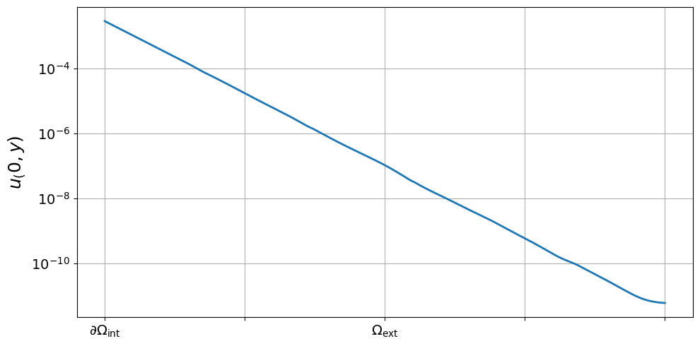
2.4. Solution Analysis#
The computed solution demonstrates the effectiveness of the PML approach:
2.4.1. Physical Behavior#
Interior region (\(\Omega_{\text{int}}\)): The solution exhibits natural wave propagation behavior
PML region (\(\Omega_{\text{ext}}\)): Artificial damping is applied through complex coordinate transformation
A rigorous parameter sensitivity analysis is done in Chapter 3 of the Bachelor Thesis
x_vals = np.linspace(1, 2, 200)
y_fixed = 0
points = [(x, y_fixed) for x in x_vals]

abs_vals = [abs(solution(mesh(x, y))) for (x, y) in points]

plt.figure(figsize=(10, 5))
plt.plot(x_vals, abs_vals, linewidth=2)


# Achsenbeschriftung
plt.grid(True)

# Benutzerdefinierte x-Achse
x_left = x_vals[0]
x_right = x_vals[-1]
tick_positions = np.linspace(x_left, x_right, 5)
tick_labels = [""] * 5
tick_labels[0] = r"$\partial\Omega_{\mathrm{int}}$"
tick_labels[2] = r"$\Omega_{\mathrm{ext}}$"
plt.xticks(tick_positions, tick_labels, fontsize=14)
plt.yticks(fontsize=14)
plt.yscale("log")
plt.ylabel(r"${u}_(0,y)$", fontsize=18)
plt.tight_layout()
#plt.savefig("pml_decay_plot.png", dpi=300)
plt.show()