PMLs in Star-shaped coordinates

3. PMLs in Star-shaped coordinates#

from ngsolve import *
from netgen.geom2d import *
from nonlin_arnoldis import *
from ngsolve.webgui import Draw
import numpy as np
from netgen.occ import *
import matplotlib.pyplot as plt
from matplotlib.pyplot import plot,show,xlim,ylim,legend
from fem1d import geo1d

maxh = 0.5    #mesh-size
order = 4     #fem order
shift = 4-0.5j      #shift for Arnoldi algorithm

#omega has to be =1 for EV problem
omega = 1
center = (0,0)    #center of inner circle
center2 = (+0.2,0.3)
R = 1           #radius of inner circle
R2 = 0.2

#params for complex scaling
alpha = 5.0
gamma = 0.0

#create geometry
circle = Circle(center, R).Face()
circle.edges.name = 'Gamma'
circle.faces.name ='inner'

circle2 = Circle(center2, R2).Face()


geo = OCCGeometry(circle-circle2, dim=2)
#geo = OCCGeometry(circle, dim=2)


#create mesh
mesh = Mesh(geo.GenerateMesh(maxh=maxh))
mesh.Curve(2*order)

Draw(mesh, order=order)

BaseWebGuiScene

3.1. Complex Scaling#

For this example we implement a frequency-dependent complex scaling transformation:

\[\sigma(\omega) := 1 + \frac{\alpha}{\gamma - i\omega} \in \mathbb{C}\]

where \(\alpha, \gamma \in \mathbb{R}\).

3.2. Tensor Product Discretization#

We implement the star-shaped PML using a tensor-product finite element method (see Chapter 5 of the Bachelor Thesis) for the exterior domain that combines:

Inherited surface discretization of the interior 2D finite elements on the physical domain
Radial 1D finite elements for the exterior unbounded region

This approach allows us to handle the unbounded exterior efficiently without explicit meshing.

n = specialcf.normal(2)
v = CoefficientFunction((x,y))          #changing x,y alteres middle point of complex scaling   

mesh1d = Mesh(geo1d(0,1).GenerateMesh(maxh=0.1))
fes1d = H1(mesh1d,order=order,complex=True)

N = fes1d.ndof

Gamma = mesh.Boundaries('Gamma')

fes_int = H1(mesh,order=order,complex=True)
fes_surf = H1(mesh,order=order,complex=True,definedon=Gamma)

fes = ProductSpace(fes_int,*( (N-1)*[fes_surf]) )
print("Number of Dofs ", fes.ndof)

Number of Dofs  5734

u,u_ = fes1d.TnT()

fem1d_mass_surf = array(BilinearForm(u*u_*ds('left')).Assemble().mat.ToDense())

fem1d_mass = array(BilinearForm(u*u_*dx).Assemble().mat.ToDense())
fem1d_mass_x = array(BilinearForm(x*u*u_*dx).Assemble().mat.ToDense())
fem1d_mass_xx = array(BilinearForm(x*x*u*u_*dx).Assemble().mat.ToDense())

fem1d_drift = array(BilinearForm(grad(u)*u_*dx).Assemble().mat.ToDense())
fem1d_drift_x = array(BilinearForm(x*grad(u)*u_*dx).Assemble().mat.ToDense())
fem1d_drift_xx = array(BilinearForm(x*x*grad(u)*u_*dx).Assemble().mat.ToDense())

fem1d_laplace = array(BilinearForm(grad(u)*grad(u_)*dx).Assemble().mat.ToDense())
fem1d_laplace_x = array(BilinearForm(x*grad(u)*grad(u_)*dx).Assemble().mat.ToDense())
fem1d_laplace_xx = array(BilinearForm(x*x*grad(u)*grad(u_)*dx).Assemble().mat.ToDense())

used dof inconsistency
(silence this warning by setting BilinearForm(...check_unused=False) )

3.3. Complex Scaled Sesquilinear Forms#

Now we assemble the complex scaled sesquilinear forms for star-shaped coordinates, which are derived in Chapter 6 of the Bachelor Thesis.

sig_1 = alpha/(gamma - omega*1j)
sig_a = alpha/(gamma - omega*1j+alpha)


S_rad_1 = (fem1d_laplace - sig_a*fem1d_laplace + 2*fem1d_laplace_x + fem1d_laplace_xx + sig_1*fem1d_laplace_xx
            - 1/4*fem1d_mass - 1/4*sig_1*fem1d_mass
            -1/2*fem1d_mass_surf) #fertig

S_rad_2 = 1*fem1d_mass + sig_1 * fem1d_mass    #fertig

D_rad = fem1d_drift + fem1d_drift_x + sig_1 * fem1d_drift_x   #fertig

M_rad = (fem1d_mass + sig_1* fem1d_mass
        + 2*fem1d_mass_x + 4 * sig_1 * fem1d_mass_x + 2*sig_1**2 * fem1d_mass_x
        + fem1d_mass_xx + 3*sig_1 * fem1d_mass_xx + 3*sig_1**2*fem1d_mass_xx + sig_1**3 * fem1d_mass_xx) #fertig

ds_g = ds(definedon=Gamma)
p,q = fes.TnT()
p_int,q_int = p[0],q[0]

S_form =(
        #interior
        grad(p_int)*grad(q_int)*dx

        #exterior
        +sum(S_rad_1[i,j]*1/(n*v)*p[j]*q[i]*ds_g
           for i in range(N) for j in range(N) if abs(S_rad_1[i,j])>0)
        -sum(D_rad.T[i,j]*1/(n*v)*(v*p[j].Trace().Deriv())*q[i]*ds_g               #be aware fem matrix is transposed, so counterintuitive one is transposed
           for i in range(N) for j in range(N) if abs(D_rad[i,j])>0)
        -sum(D_rad[i,j]*1/(n*v)*p[j]*(v*q[i].Trace().Deriv())*ds_g
           for i in range(N) for j in range(N) if abs(D_rad[i,j])>0)
        +sum(S_rad_2[i,j]*(v*v)/(n*v)*p[j].Trace().Deriv()*q[i].Trace().Deriv()*ds_g
           for i in range(N) for j in range(N) if abs(S_rad_2[i,j])>0)
        -sum(S_rad_2[i,j]*1/(2*n*v)*((p[j].Trace().Deriv()*v)*q[i]+p[j]*(v*q[i].Trace().Deriv()))*ds_g
           for i in range(N) for j in range(N) if abs(S_rad_2[i,j])>0))

M_form =( 
        #interior
        -omega **2 * p_int*q_int*dx

        #exterior
        - omega**2 * sum(M_rad[i,j]*(n*v)*p[j]*q[i]*ds_g
           for i in range(N) for j in range(N) if abs(M_rad[i,j])>0))

3.4. Complex Scaled Helmholtz Equation#

3.4.1. Problem Formulation#

We solve the complex scaled Helmholtz equation:

\(-\Delta u - \omega^2 u = f \quad \text{in } \Omega_{\text{int}}\)

with the star-shaped PML providing transparent boundary conditions on \(\Gamma\).

The right-hand side \(f\) represents a localized excitation in the interior domain.

f = exp(-5**2*((x+0.2)**2 + (y+0.3)**2))

m_star = BilinearForm(S_form + M_form, symmetric=True).Assemble()
b = LinearForm(f * q_int * dx).Assemble()


gfp = GridFunction(fes)
gfp.vec.data = m_star.mat.Inverse(freedofs=fes.FreeDofs()) * b.vec

Draw(gfp.components[0], mesh, animate_complex = True, order = 6)

BaseWebGuiScene

3.4.2. Interior Behavior#

The solution exhibits natural wave propagation in the interior domain \(\Omega_{\text{int}}\).

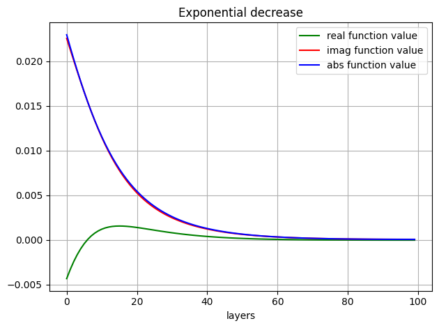
3.4.3. Exterior Damping#

In the exterior region, the complex scaling transformation introduces exponential damping, effectively absorbing outgoing waves.

Since we use a tensor-product approach without explicitly meshing the exterior, we cannot directly visualize the full 3D behavior. Instead, we examine the radial decay profile along a specific direction to demonstrate the exponential damping characteristic of the PML.

snapshot=[]
p1, p2 = center[0], center[1]
mp = mesh(p1+R,p2,0, BND)
for i in range(N):
    snapshot.append(gfp.components[i](mp))      
     
solution= GridFunction(fes1d)
solution.vec.FV().NumPy()[:] = snapshot

M = 100
xvals = np.linspace(0, 1, M)
yvals_real = [np.real(solution(x)) for x in xvals]
yvals_imag = [np.imag(solution(x)) for x in xvals]
yvals_abs = [np.abs(solution(x)) for x in xvals]

plt.plot(yvals_real, label="real function value", color = 'green')
plt.plot(yvals_imag, label="imag function value", color = 'red')
plt.plot(yvals_abs, label="abs function value", color = 'blue')
plt.xlabel('layers')
plt.legend()
plt.title("Exponential decrease")
plt.grid(True)
plt.tight_layout()
plt.show()

_images/c5929a0415d64a432c676462e01003e417b7d998b9e1cf3f0238dda4be82f950.png

3.5. Eigenvalue Problem#

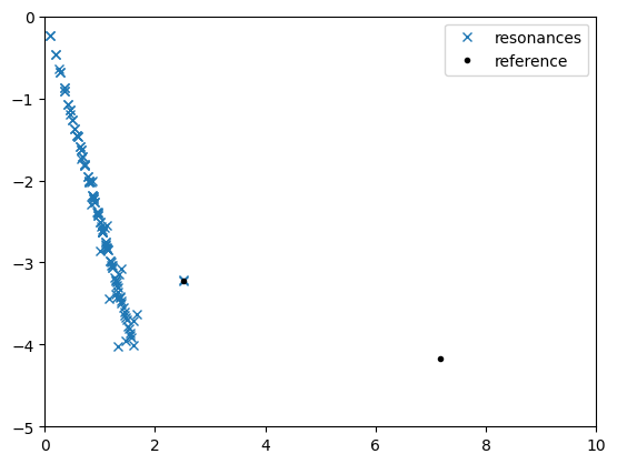
3.5.1. Resonance Computation#

To validate the correctness of our star-shaped PML method, we solve the corresponding eigenvalue problem.

3.5.2. Reference Solution#

Since our computational domain contains a circular scatterer (the inner circle), a subset of the computed spectrum must match the roots of Hankel functions - these are the analytical resonances for scattering by a circular obstacle.

3.5.3. Stability Analysis via Eigenvalues#

We begin by recalling the homogeneous Helmholtz problem:

\[-\Delta u(\mathbf{x}) - \omega^2u(\mathbf{x}) = 0\]

If, for a given frequency \(\omega\), there exists a non-trivial function \(u_\omega\) that solves this equation, we call \(\omega\) an eigenfrequency with respective eigenfunction \(u_\omega\).

Assuming that there exists a complete system of orthonormal eigenfunctions \(u_{\omega_n}, n\in \mathbb{N}_0\) of the operator \(-\Delta\) with suitable boundary conditions, then the solution can be decomposed as:

\[u(\mathbf{x}) = \sum_{n= 0}^\infty \frac{(f, u_{\omega_n})}{\omega_n^2-\omega^2}u_{\omega_n}(\mathbf{x})\]

As the inverse Fourier transformation yields exponential factors \(e^{-i \omega_n t}\), the imaginary parts of the eigenfrequencies determine the asymptotic behavior of the time-domain solution. The same theory can be applied in the discretized framework, where the decomposition into basis functions is guaranteed since the solution belongs to the finite element space.

For detailed theoretical background, see Section 7. of the Bachelor Thesis.

S = BilinearForm(S_form, symmetric = True).Assemble()
M = BilinearForm(M_form, symmetric = True).Assemble()

gf = GridFunction(fes,multidim=120)

#lam = sqrt(array(ArnoldiSolver(S.mat,M.mat,freedofs=fes.FreeDofs(),vecs=list(gf.vecs),shift=shift**2)))
lam = np.sqrt(np.array(PolyArnoldiSolver([S.mat,M.mat],shift**2,300,nevals=120,vecs=gf.vecs,inversetype='sparsecholesky',freedofs=fes.FreeDofs())))

plt.plot(lam.real,lam.imag,'x',label='resonances')

#load reference resonances from file
loaded=np.loadtxt('dhankel_1_zeros.out')
ref=(loaded[:,0]+1j*loaded[:,1])/R2

plt.plot(ref.real,ref.imag,'.k',label='reference')

plt.xlim((0,10))
plt.ylim((-5,0))
plt.legend()
#Draw(gf.components[0], animate_complex=True, order=6);            #Vizulazation of eigenfunctions

<matplotlib.legend.Legend at 0x147f39e80>